Pre-Requisite: Articulation Points
Before Biconnected Components, let's first try to understand what a Biconnected Graph is and how to check if a given graph is Biconnected or not.
A graph is said to be Biconnected if:
- It is connected, i.e. it is possible to reach every vertex from every other vertex, by a simple path.
- Even after removing any vertex the graph remains connected.
For example, consider the graph in the following figure
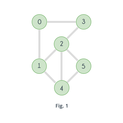
The given graph is clearly connected. Now try removing the vertices one by one and observe. Removing any of the vertices does not increase the number of connected components. So the given graph is Biconnected.
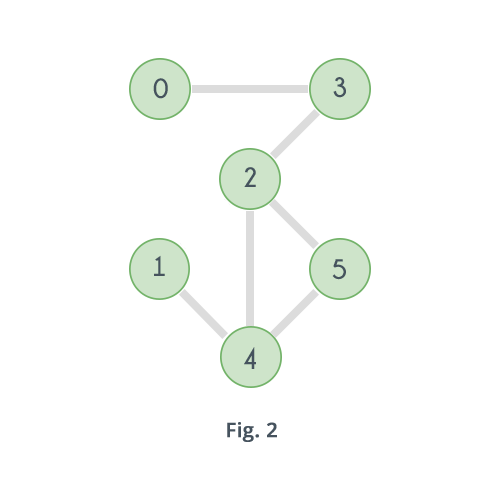
Now consider the following graph which is a slight modification in the previous graph.
Now consider the following graph which is a slight modification in the previous graph.
In the above graph if the vertex 2 is removed, then here's how it will look:
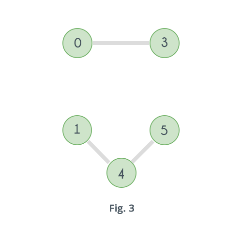
Clearly the number of connected components have increased. Similarly, if vertex 3 is removed there will be no path left to reach vertex 0 from any of the vertices 1, 2, 4 or 5. And same goes for vertex 4 and 1. Removing vertex 4 will disconnect 1 from all other vertices 0, 2, 3 and 4. So the graph is not Biconnected.
Now what to look for in a graph to check if it's Biconnected. By now it is said that a graph is Biconnected if it has no vertex such that its removal increases the number of connected components in the graph. And if there exists such a vertex then it is not Biconnected. A vertex whose removal increases the number of connected components is called an Articulation Point.
So simply check if the given graph has any articulation point or not. If it has no articulation point then it is Biconnected otherwise not. Here's the pseudo code:
time = 0
function isBiconnected(vertex, adj[][], low[], disc[], parent[], visited[], V)
    disc[vertex]=low[vertex]=time+1
    time = time + 1
    visited[vertex]=true
    child = 0
    for i = 0 to V
        if adj[vertex][i] == true
            if visited[i] == false
                child = child + 1
                parent[i] = vertex
                result = isBiconnected(i, adj, low, disc, visited, V, time)
                if result == false
                    return false
                low[vertex] = minimum(low[vertex], low[i])
                if parent[vertex] == nil AND child > 1
                    return false
                if parent[vertex] != nil AND low[i] >= disc[vertex]
                    return false
            else if parent[vertex] != i
                low[vertex] = minimum(disc[i], low[vertex])
    return true
The code above is exactly same as that for Articulation Point with one difference that it returns false as soon as it finds an Articulation Point.
The image below shows how the DFS tree will look like for the graph in Fig. 2 according to the algorithm, along with the value of the arrays and .
The image below shows how the DFS tree will look like for the graph in Fig. 2 according to the algorithm, along with the value of the arrays and .
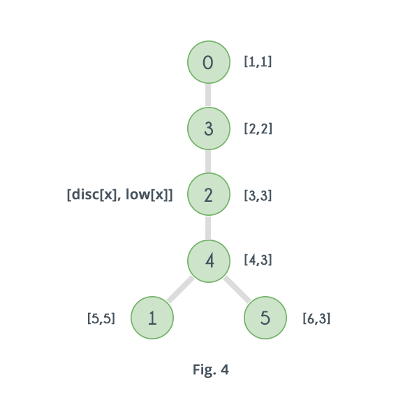
Clearly for vertex 4 and its child 1, , so that means 4 is an articulation point. The algorithm returns false as soon as it discovers that 4 is an articulation point and will not go on to check for vertices 0, 2 and 3. Value of for all vertices is just shown for clarification.
Following image shows DFS tree, value of arrays and for graph in Fig.1
Following image shows DFS tree, value of arrays and for graph in Fig.1
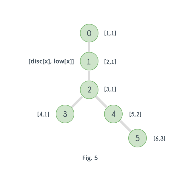
Clearly there does not exists any vertex , such that , i.e. the graph has no articulation point, so the algorithm returns true, that means the graph is Biconnected.
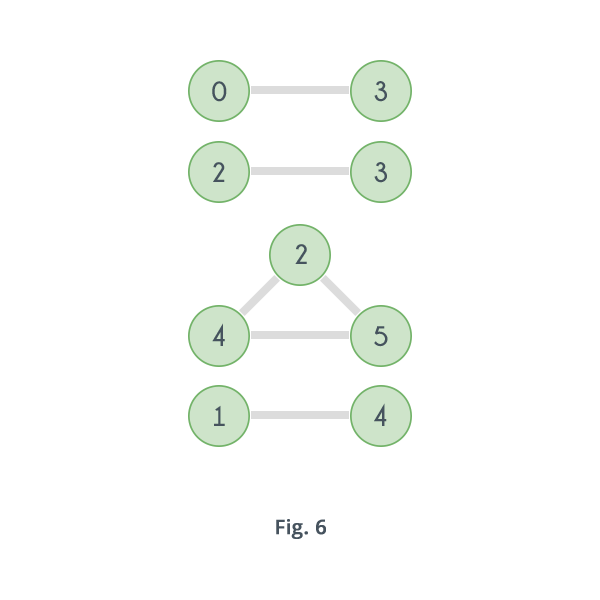
Now let's move on to Biconnected Components. For a given graph, a Biconnected Component, is one of its subgraphs which is Biconnected. For example for the graph given in Fig. 2 following are 4 biconnected components in the graph
Biconnected components in a graph can be determined by using the previous algorithm with a slight modification. And that modification is to maintain a Stack of edges. Keep adding edges to the stack in the order they are visited and when an articulation point is detected i.e. say a vertex has a child such that no vertex in the subtree rooted at has a back edge () then pop and print all the edges in the stack till the is found, as all those edges including the edge will form one biconnected component.
time = 0
function DFS(vertex, adj[][], low[], disc[], parent[], visited[], V, stack)
    disc[vertex]=low[vertex]=time+1
    time = time + 1
    visited[vertex]=true
    child = 0
    for i = 0 to V
        if adj[vertex][i] == true
            if visited[i] == false
                child = child + 1
                push edge(u,v) to stack
                parent[i] = vertex
                DFS(i, adj, low, disc, visited, V, time, stack)
                low[vertex] = minimum(low[vertex], low[i])
                if parent[vertex] == nil AND child > 1
                    while last element of stack != (u,v)
                        print last element of stack
                        pop from stack
                    print last element of stack
                    pop from stack
                if parent[vertex] != nil AND low[i] >= disc[vertex]
                    while last element of stack != (u,v)
                        print last element of stack
                        pop from stack
                    print last element of stack
                    pop from stack
            else if parent[vertex] != i AND disc[i] < low[vertex]
                low[vertex] = disc[i]
                push edge(u,v) to stack

fuction biconnected_components(adj[][], V)
    for i = 0 to V
        if visited[i] == false
            DFS(i, adj, low, disc, parent, visited, V, time, stack)
            while stack is not empty
                print last element of stack
                pop from stack
Let's see how it works for graph shown in Fig.2.
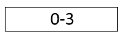
First it finds is false so it starts with vertex 0 and first discovers the edge 0-3 and pushes it in the stack.
First it finds is false so it starts with vertex 0 and first discovers the edge 0-3 and pushes it in the stack.
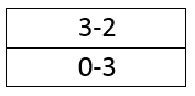
Then with 3 it finds the edge 3-2 and pushes that in stack
With 2 it finds the edge 2-4 and pushes that in stack
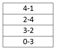
For 4 it first finds edge 4-1 and pushes that in stack
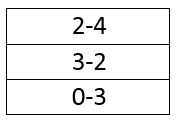
It then discovers the fact that i.e. discovers that 4 is an articulation point. So all the edges inserted after the edge 4-1 along with edge 4-1 will form first biconnected component. So it pops and print the edges till last edge is 4-1 and then prints that too and pop it from the stack
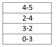
Then it discovers the edge 4-5 and pushes that in stack
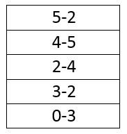
For 5 it discovers the back edge 5-2 and pushes that in stack
After that no more edge is connected to 5 so it goes back to 4. For 4 also no more edge is connected and also .
Then it goes back to 2 and discovers that , that means 2 is an articulation point. That means all the edges inserted after the edge 4-2 along with the edge 4-2 will form the second biconnected component. So it print and pop all the edges till last edge is 4-2 and then print and pop that too.
Then it goes to 3 and discovers that 3 is an articulation point as so it print and pops till last edge is 3-2 and the print and pop that too. That will form the third biconnected component.
Now finally it discovers that for edge 0-3 also so it pops it from the stack and print it as the fourth biconnected component.
Then it checks value of other vertices and as for all vertices it is true so the algorithm terminates.
So ulitmately the algorithm discovers all the 4 biconnected components shown in Fig.6.
Time complexity of the algorithm is same as that of DFS. If is the number of vertices and is the number of edges then complexity is .

Không có nhận xét nào:
Đăng nhận xét